FPGA to GPU over 100G RoCE: a live beamforming demo

I’ve always wanted to work on a project that bridged FPGAs with GPUs. Well this post is about my first project that does exactly that. I’m going to write about the latest Opsero ref design, qsfp28-fmc-rocelet, and the demo built into it. At its core is rocelet, a RoCE v2 (RDMA over Converged Ethernet) engine that you’ll find in its own repository, released under the MIT license so that you can drop it into your own designs. The reference design wraps that engine into a complete 100G system on the AMD Kintex UltraScale+ KCU116 with our 2x QSFP28 FMC (OP120). All of this is open source and doesn’t require any paid licenses. On top of that we built a phased-array beamforming demo: the FPGA streams the samples of a simulated 8 x 8 antenna array over 100G RoCE v2 straight into the memory of an NVIDIA GPU, and the GPU turns them into a live picture of where the signals are coming from.

In most of this post I’ll explain how the demo works, what it’s doing and how to drive it. I have to admit it’s a bit of a long read (sorry), but it’s a big demo - much bigger than most of my past projects - with lots of moving parts.

Why beamforming?

My goal for this project was a demo that would show off the 2x QSFP28 FMC running at the full 100 Gbps line rate, and do something that resembles a real-world application. The hard part of any 100G demo is that a single link carries so much data (12.5 GB/s) that it’s hard to find a real source or a real sink for it. Not many devices produce that much data, and not many devices can take it in.

The idea of RDMA into a GPU came from one of my contacts at AMD. GPUs can actually consume that kind of data rate, and a NIC that supports GPUDirect RDMA can write network data straight into GPU memory. That solved the sink. For the source, a few of my professional contacts pointed me towards beamforming. A digital phased array has one receiver channel per antenna element, so even a modest array produces a torrent of IQ samples that all have to be processed together, which is exactly the kind of job a GPU is good at. I don’t have an RFSoC or any antennas (yet), so the IQ data had to be simulated inside the FPGA. Those constraints led to this setup:

KCU116 + OP120 → QSFP28 AOC → NVIDIA ConnectX-6 Dx NIC → NVIDIA RTX PRO 4000 Blackwell GPU

The FPGA simulates the IQ signals “received” by an 8 x 8 planar antenna array, sends them over the 100G RoCE v2 link to the ConnectX-6 Dx, and the NIC writes them straight into GPU memory. A Holoscan application on the host does the beamforming on the GPU and draws the result on a monitor. The video below is a 20 second clip of the demo nulling a jammer (more on that later).

The hardware

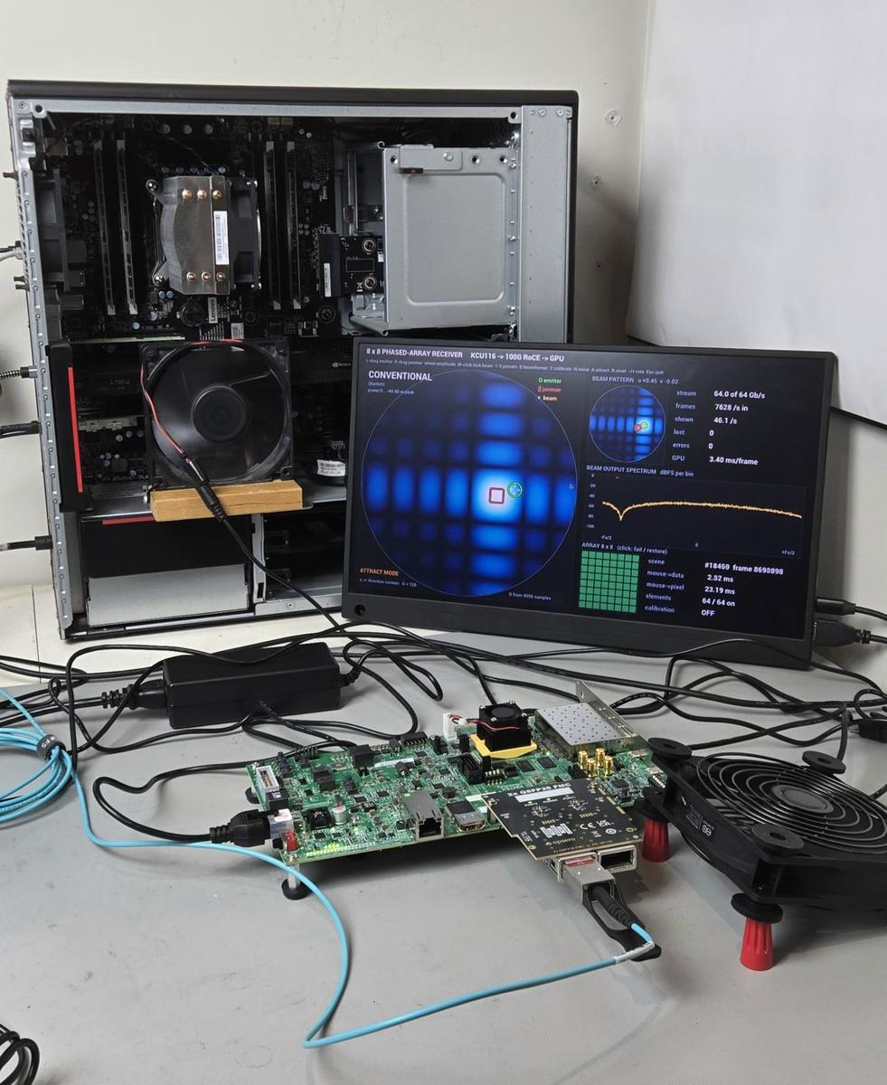
The photo at the top of this post shows the setup: the KCU116 with the 2x QSFP28 FMC on its FMC connector in the foreground, the test host behind it with its side panel off, and the demo running on a portable monitor. The aqua cable is the 100G AOC running from QSFP28 port 0 of the FMC to the NIC in the host.

The P520 is an older machine, and I chose it because it was easy to get my hands on. That turned out to be the main limit of the demo, as I’ll explain further down.

Two quick primers

RDMA and RoCE v2

When a normal network application receives data, the NIC hands the packets to the operating system, the kernel processes them and copies the data into the application’s buffers. The CPU touches every packet. At 100 Gbps that’s a losing battle: on our test host, a plain Linux UDP receiver was clean to only 8 Gbps.

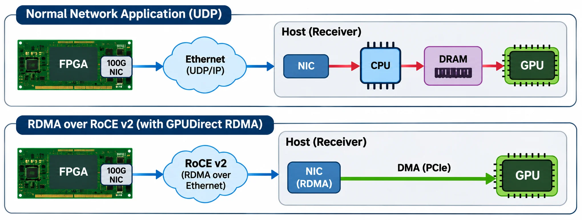
RDMA (remote direct memory access) takes the CPU out of that path. The receiving side registers a region of memory with its NIC, tells the sender where that region is, and from then on the sender can write into it directly. The NIC handles the transport in hardware and places the data in memory with DMA; no CPU copies anything. RoCE v2 is RDMA carried over ordinary Ethernet, inside UDP/IP packets, so it works with standard 100G NICs and cables. And with GPUDirect RDMA, the registered memory can be GPU memory, so the NIC writes the data over PCIe straight into the GPU. That’s what happens in this demo: the samples go from the FPGA fabric to the GPU’s memory without a single CPU copy.

The illustration below compares the two paths. With a normal UDP application, the data goes from the NIC through the CPU and host memory (DRAM) before it gets to the GPU. With RoCE v2 and GPUDirect RDMA, the NIC writes it over PCIe directly into GPU memory.

Beamforming

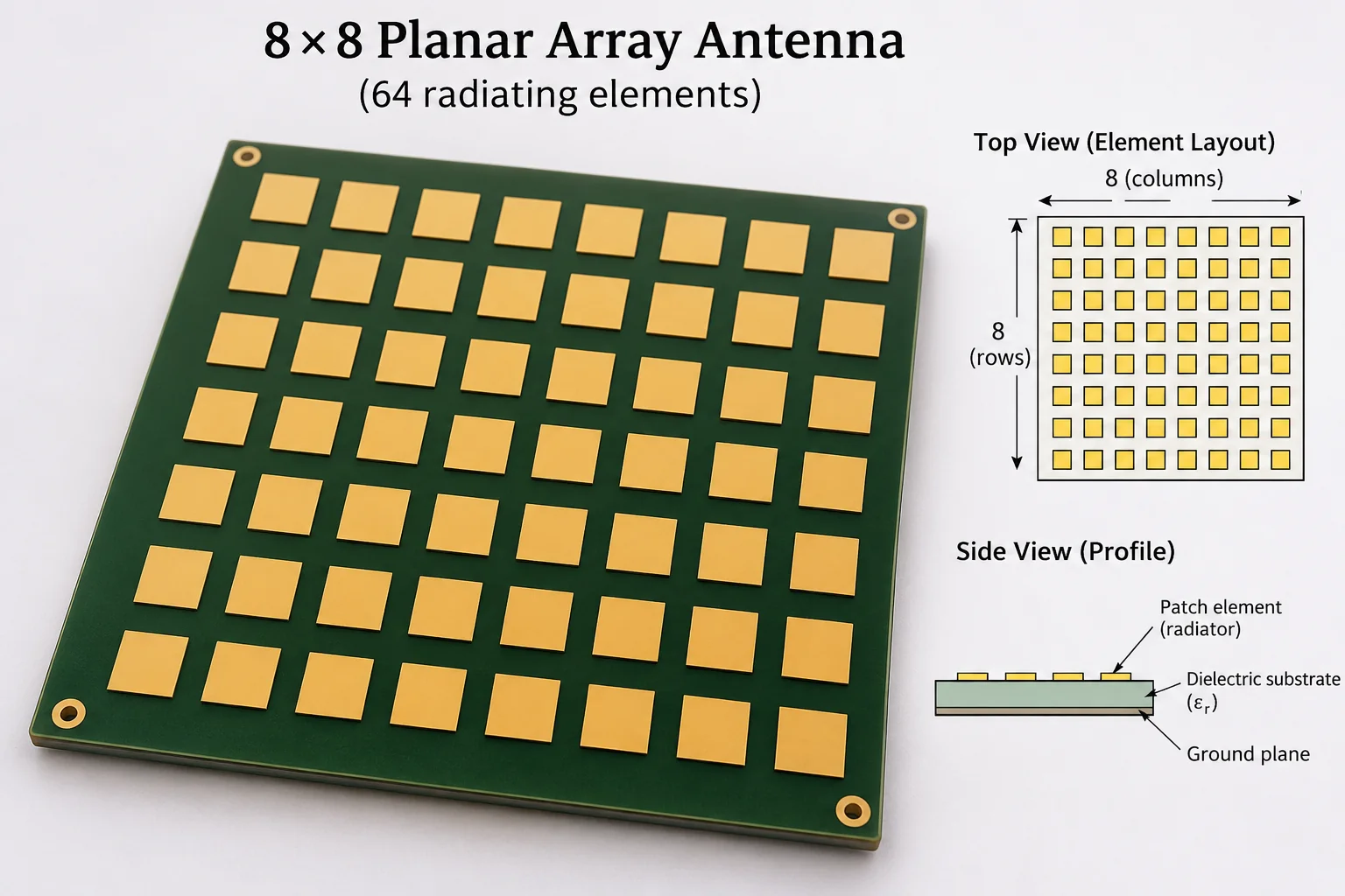
Imagine an array of 64 antennas laid out in an 8 x 8 grid, half a wavelength apart, and a radio signal arriving from some direction. The wave reaches each antenna at a slightly different time, and for a narrowband signal that shows up as a different phase at each element. The pattern of phase shifts across the array depends only on the direction the wave came from. The illustration below shows what such an array can look like: 64 square patch antennas on a printed circuit board, each one with its own receiver channel behind it.

So if you want to listen in one particular direction, you take each element’s samples, undo the phase shift that a wave from that direction would have caused, and add all 64 together. Signals from that direction add up in phase, and signals from everywhere else partly cancel. That’s a beam, and you’ve “pointed” it without moving anything: it’s just math on the samples. Now do that for every direction on a grid, measure the power in each beam, and you have a picture of where the signals are coming from, a sort of “radio camera”. That’s the main display of the demo.

The demo shows two ways of forming the beams:

• Conventional (also called Bartlett or delay-and-sum) is exactly what I described above. It’s simple and robust, but an 8 x 8 array is small, so its beams are wide, and every beam has sidelobes: weaker “echoes” of the main beam in other directions, about 13 dB down. A strong signal leaks into the beams pointed elsewhere, and can bury a weaker signal.
• MVDR (minimum variance distortionless response, also called Capon) is adaptive. For each direction it computes a set of weights from the data itself, so that the beam has unit gain in the look direction and lets through as little power as possible from everywhere else. In practice that means it automatically places nulls on the other strong signals. It resolves sources that are close together, and it can suppress a jammer, but it relies on the array being calibrated.

Both start from the covariance matrix of the frame: a 64 x 64 matrix that says how the signal at every element correlates with the signal at every other element. All of the directional information is in that matrix, and the GPU computes it from every frame it processes (0.3 ms).

What the demo is doing

The diagram below shows the whole thing: the data path from the FPGA into GPU memory, and the control path from the mouse back to the FPGA. I’ll walk through it in the next few sections.

Where the IQ samples come from

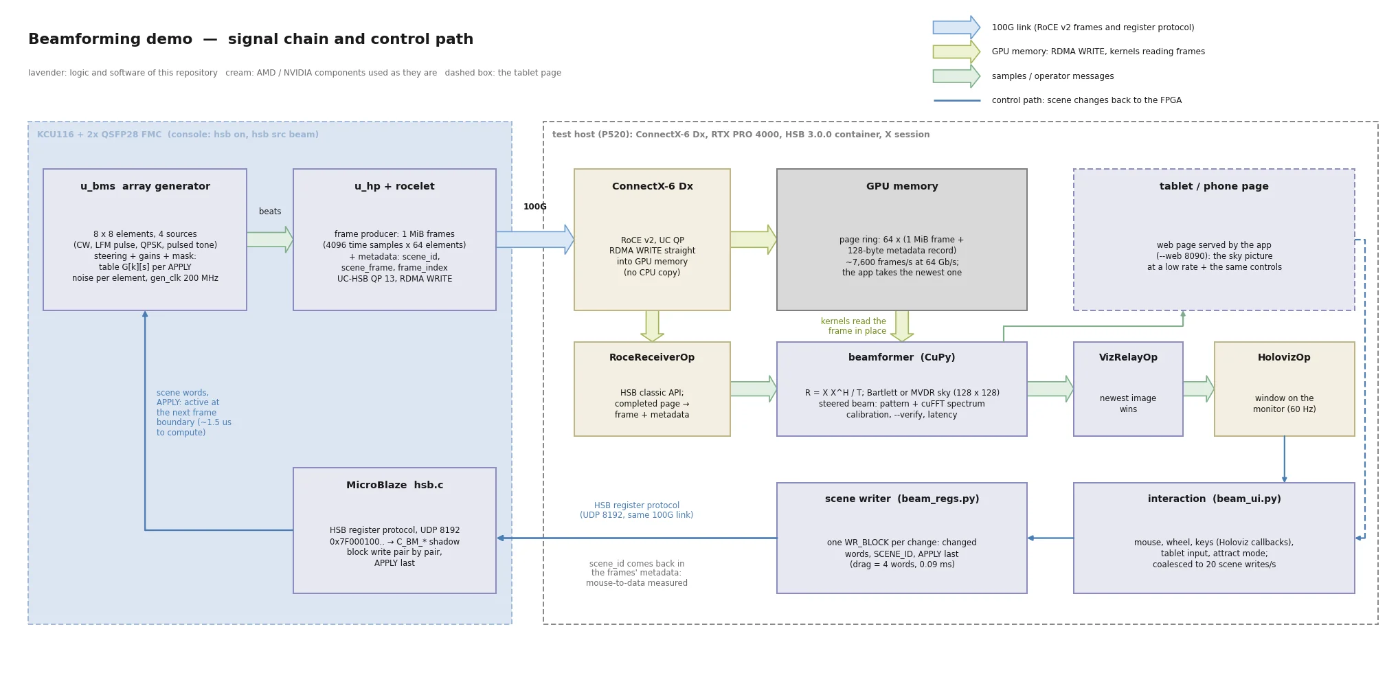
The samples are generated in the FPGA by an “array generator” written in RTL. It plays the role of the digitizer of a phased-array receiver: for every time sample, it computes what each of the 64 antenna elements would receive from up to four signal sources. Each source has a direction, an amplitude and a waveform. There are four waveforms: a CW tone, an LFM pulse (a chirp, like a radar pulse), QPSK (a noise-like communications signal) and a pulsed tone. From each source’s direction, the generator computes the phase that every element sees, sums the sources, and adds random noise to each element, as a real receiver channel would. It can also apply a gain and phase error to each element (an uncalibrated array) and disable elements (failed channels that only output noise).

The output is complex baseband (IQ) samples, 16-bit I and 16-bit Q per element per time sample. The samples are packed into 1 MiB frames, each holding 4,096 time samples from all 64 elements, plus a 128-byte metadata record that says which scene (set of source positions and settings) the frame was generated with. At 64 Gbps that’s about 7,600 frames per second, or 31.2 MS/s per element.

To be clear: this is simulated data. Nothing here is coming from real antennas. But the generator is bit-exact with a reference model in Python, so every frame that arrives at the GPU can be checked word for word, and we did exactly that (more on that below).

Where the samples go

The frames leave the FPGA through rocelet, our RoCE v2 engine, as RDMA WRITEs, through the Kintex UltraScale+ integrated 100G Ethernet MAC (CMAC, with RS-FEC) and out of QSFP28 port 0 of the 2x QSFP28 FMC. On the host, the ConnectX-6 Dx receives them and writes them straight into a ring of buffers in GPU memory.

The host side is NVIDIA’s Holoscan Sensor Bridge (HSB) software. HSB is NVIDIA’s framework for getting sensor data from an FPGA, over Ethernet, into GPU memory, and it’s built on the Holoscan SDK, NVIDIA’s framework for streaming sensor processing applications. Normally the FPGA side of HSB is NVIDIA’s own IP. In this design, the FPGA implements the device side of the HSB protocol itself (enumeration, the register protocol and the RoCE data plane), so the KCU116 shows up as an HSB device and NVIDIA’s unmodified HSB 3.0.0 host software receives the data.

Once a frame has landed in GPU memory, the beamforming application picks it up where it is. The application is a Holoscan app written in Python, with the processing done in CuPy kernels on the GPU. For each frame it processes, it computes:

1. The covariance matrix (64 x 64) from the frame’s 4,096 x 64 samples.
2. The sky map: the beam power in every direction on a 128 x 128 grid, with the conventional or MVDR beamformer.
3. The weights of one “steered” beam (the one you point with the mouse), its beam pattern over the sky, and the spectrum of that beam’s output, with a 4,096-point FFT.

Then it draws all of that in a Holoviz window on the monitor. That takes about 3.2-3.5 ms of GPU time per frame with the conventional beamformer and about 6 ms with MVDR. The display refreshes at 60 Hz, so the app beamforms and shows about 45 frames per second and only counts the others; at 64 Gbps about 7,600 frames per second arrive in GPU memory.

What you’re looking at

The image below is a screenshot of the application window. Here it’s showing preset 3: two CW emitters, one beamwidth apart, with the conventional beamformer.

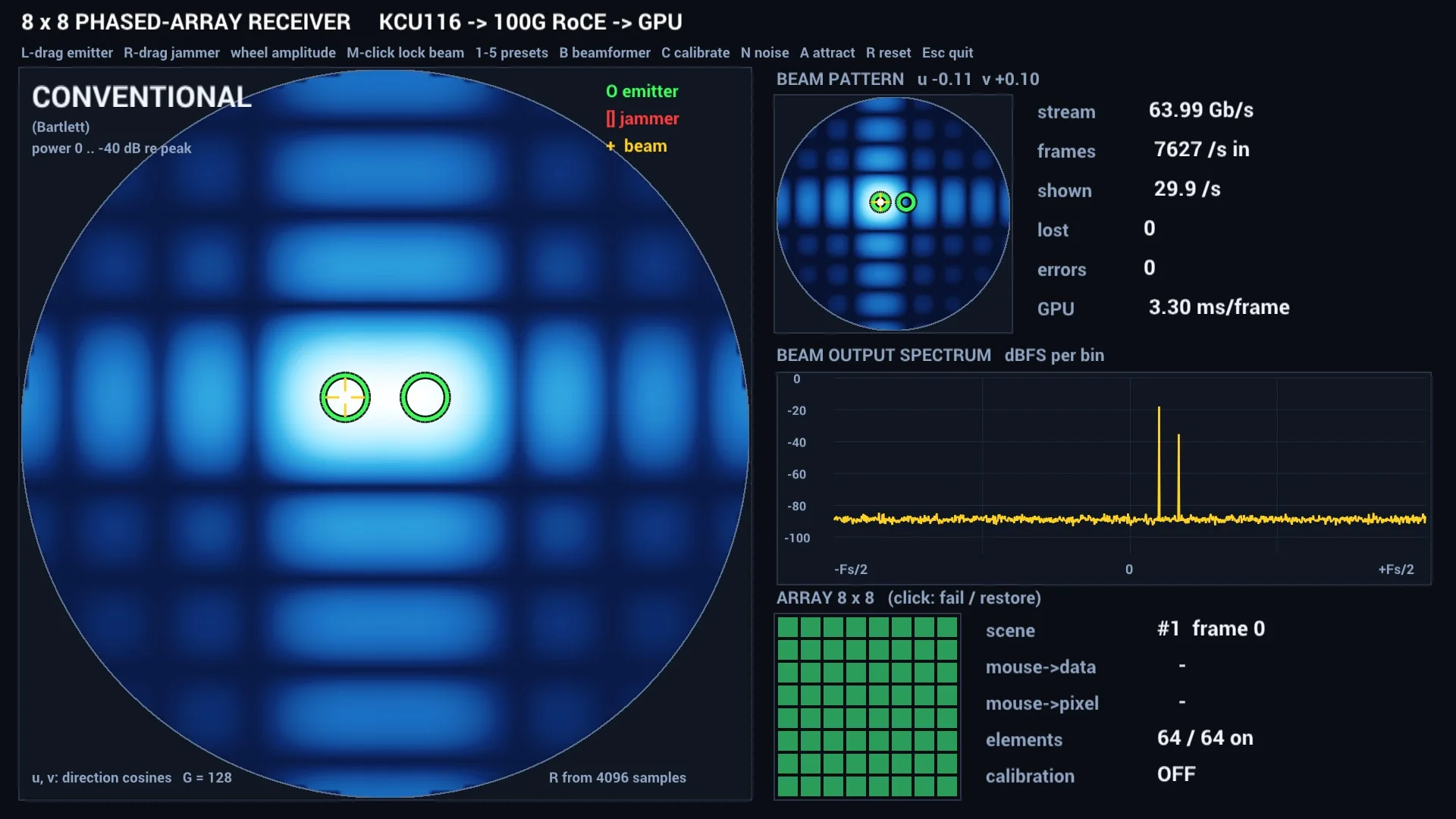
The big disc on the left is the “sky”. It’s the hemisphere in front of the array, flattened into a circle: the centre is straight ahead of the array (boresight), the edge is the horizon, left-right runs along the array’s rows and up-down along its columns. (Technically, the axes are the direction cosines u and v.)

The key to reading the display is to understand that it contains two different kinds of information:

• The markers are the known positions. Green circles are emitters (the wanted signals) and red squares are jammers (strong interferers). They’re drawn where the sources really are: the application told the FPGA where to put them, and every frame’s metadata says which scene it was generated with, so the markers are the ground truth for that frame. The GPU doesn’t compute them.
• The blue shading is what the GPU computes. Each of the 128 x 128 pixels inside the disc is the power the array measures when a beam is pointed in that direction, computed from the frame’s raw samples alone: dark is weak, bright is strong. It’s the array’s estimate of where the signals are.

The difference between the two is the point of the demo. In the screenshot above, the conventional beamformer can’t separate the two emitters: they’re closer together than its beam is wide, so they merge into one bright blob. The regular grid of blue rectangles around it is the sidelobe pattern of an 8 x 8 array. Press B to switch to MVDR and the blob splits into two sharp points.

The yellow crosshair is the steered beam. It follows the mouse pointer (a middle click locks it on the nearest source). The panels on the right are computed for that beam: the beam pattern (top right) shows how sensitive that beam is in every direction, and the beam output spectrum (middle right) shows what that beam hears. In the screenshot, the beam is on the left emitter but the spectrum shows two tones, because the conventional beam is too wide to keep the second emitter out. The array panel (bottom right) shows the 64 elements, and you can click one to fail it. The tiles show the stream rate, frames received and shown per second, lost frames, GPU time per frame and the latency of your last mouse action.

Moving the sources: the control path

Here’s the part I like the most. With the left mouse button you can drag an emitter anywhere on the sky, and with the right button, a jammer. The scroll wheel changes a source’s amplitude, the number keys 1-5 load presets, and - / + change the stream rate between 1 and 80 Gbps while it runs.

When you drag a source, the application doesn’t move a marker on the screen; it changes the scene in the FPGA. Every mouse move (coalesced to 20 updates per second) becomes a single block-write of four 32-bit registers: the new u and v of the source, a new scene ID and an APPLY bit. That write goes out over the HSB register protocol (UDP port 8192), from the ConnectX-6 Dx, over the same 100G link and the same cable, in the opposite direction to the data. In the FPGA, rocelet passes the register packets to the MicroBlaze, which writes the values into the array generator’s shadow registers. On APPLY, the generator computes the steering phases for the new scene (about 1.5 µs) and switches to it at the next frame boundary, so no frame ever mixes two scenes. The first frame of the new scene carries the new scene ID in its metadata, and when it arrives in GPU memory, the application knows how long the round trip took.

That time is shown in the tiles as mouse→data, and it’s about 1.5-2.7 ms: from the mouse event, out to the FPGA, and back in GPU memory as samples from the new scene. Mouse→pixel is about 23 ms, and most of that is the 60 Hz display.

The application also serves a web page (on port 8090) that you can open on a tablet or phone on the same LAN. It shows the same sky map and has the same controls, so you can drag the sources around with a finger.

Conventional vs MVDR: nulling a jammer

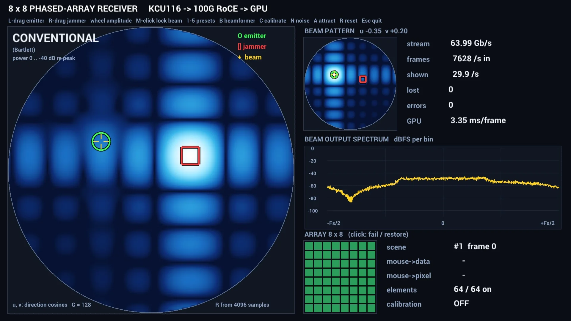
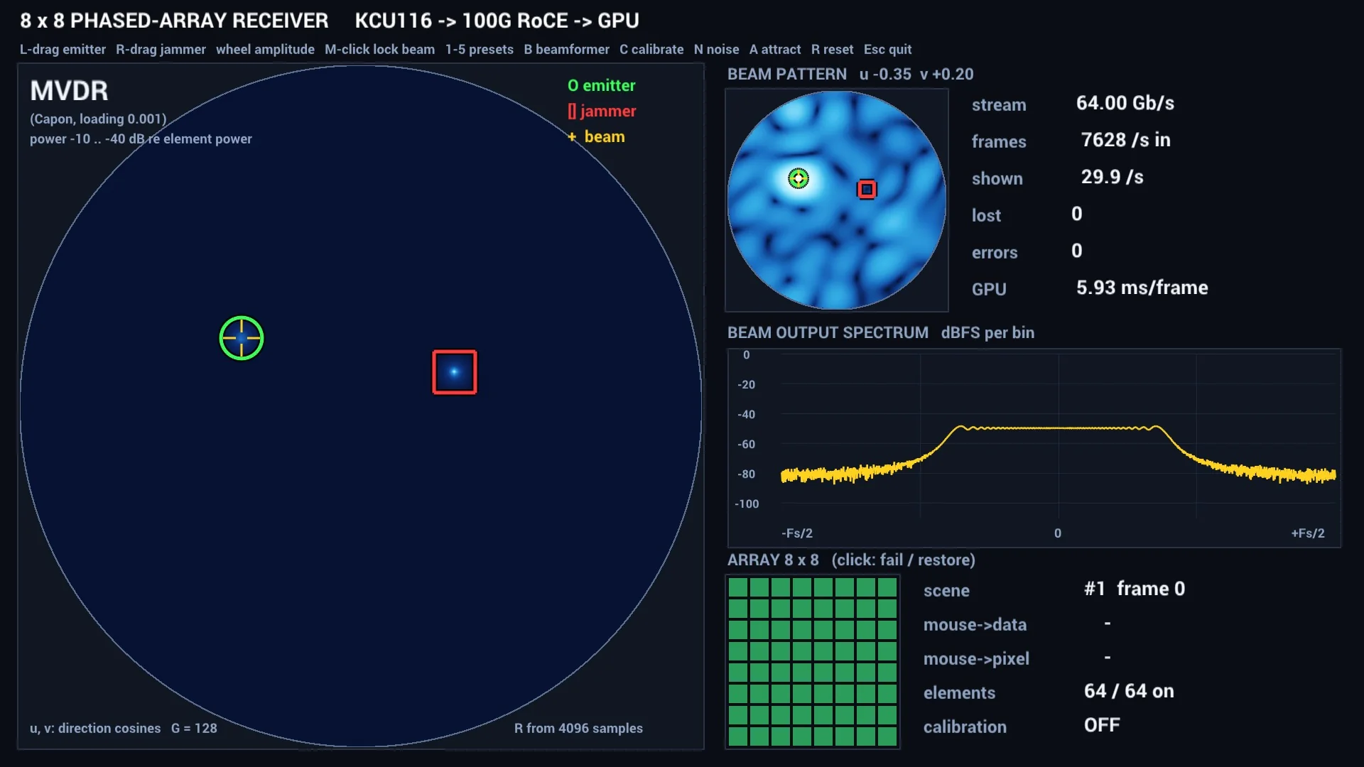
The two screenshots below show preset 2: a radar-like LFM emitter (green circle) and a QPSK jammer 18 dB stronger (red square). With the conventional beamformer (left), the jammer’s main lobe and sidelobes cover the whole sky, and the emitter is invisible. Even with the beam pointed right at the emitter, the spectrum shows mostly the jammer’s wideband hump. With MVDR (right), both sources collapse to points, the beam pattern grows a notch where the jammer is, and the spectrum becomes the flat band of the LFM pulse, about 30 dB above the noise floor. The jammer has been nulled, adaptively, from the covariance matrix of each frame. This is what the video near the top of the post shows.

The videos

I’ve put up five short videos on YouTube. Each one runs a preset for 10 seconds with the conventional beamformer and then switches to MVDR (or turns on calibration), and the video descriptions explain what’s happening:

• One emitter, conventional vs MVDR: the main lobe and sidelobe grid of an 8 x 8 array, and what MVDR does to a single source.
• Nulling a jammer with MVDR: preset 2, the video embedded above.
• Resolving two sources one beamwidth apart: preset 3, the screenshot above, and how MVDR separates the two emitters.
• Phased array with failed elements: six of the 64 elements disabled, and what that does to the sidelobes.
• Array calibration live: random gain and phase errors on every element, removed by a calibration that the GPU estimates from the data.

Ideally, this would be an RFSoC

If you wanted to do this with real signals, the KCU116 is not the board you’d pick. In this configuration, the 2x QSFP28 FMC occupies the KCU116’s only FMC connector, so there’s no practical way to get real antenna data into it. You’d do this with an RFSoC board like the AMD ZCU216, whose RF-ADCs can digitize the antenna elements directly, and a real planar antenna array (probably a smaller one than 8 x 8, unless you have a lot of ADC channels). The FPGA side of the data path would be the same: samples into rocelet, out over 100G and into the GPU.

But the point of this project wasn’t to build a radar. I needed a platform to develop the RoCE v2 engine on and to actually test it on hardware, with a real NIC and a real GPU at the other end, and I wanted a demo for the 2x QSFP28 FMC at the same time. The KCU116, with the integrated 100G MAC (CMAC) of its Kintex UltraScale+, gave me all of that.

The rocelet RoCE v2 engine

So why did we write our own RoCE v2 engine? AMD already has one, the ERNIC IP, which implements a full RoCE v2 stack. But it’s large (about 42k LUTs plus the interconnect, buffers and queues it needs on a Kintex UltraScale+) and it’s paid, licensed IP. Most FPGA RoCE applications that I’ve come across stream data between an FPGA and a host or a GPU over a point-to-point link, and they need only a small part of the protocol. rocelet implements that part, in about 21k LUTs.

• Written in vendor-neutral SystemVerilog, with a 512-bit AXI4-Stream interface to the MAC at the CMAC user clock (322 MHz for 100GbE).
• RC (reliable connection) requester: RDMA WRITE, WRITE with immediate, SEND, SEND with immediate, multi-packet messages, and go-back-N retransmission from an on-chip retransmit ring.
• RC responder: RDMA WRITEs and SENDs from the host into FPGA memory, and RDMA READs of FPGA memory by the host, with full duplicate and NAK handling.
• IPv4/UDP framing, ICRC on TX and RX, path MTU 256-4096, 802.3x PAUSE honoured and generated, and a built-in ARP/ICMP responder.
• A Holoscan Sensor Bridge mode (the UC queue pair that this demo uses).
• Out-of-band queue pair setup: a small host helper based on libibverbs exchanges the queue pair numbers, PSNs, rkeys and buffer addresses. There’s no in-band connection manager.

The engine has some known limitations: it’s IPv4 only, it doesn’t do atomics, and it answers RDMA READs but doesn’t issue them. The rocelet docs cover its architecture, interface, register map and how to integrate it.

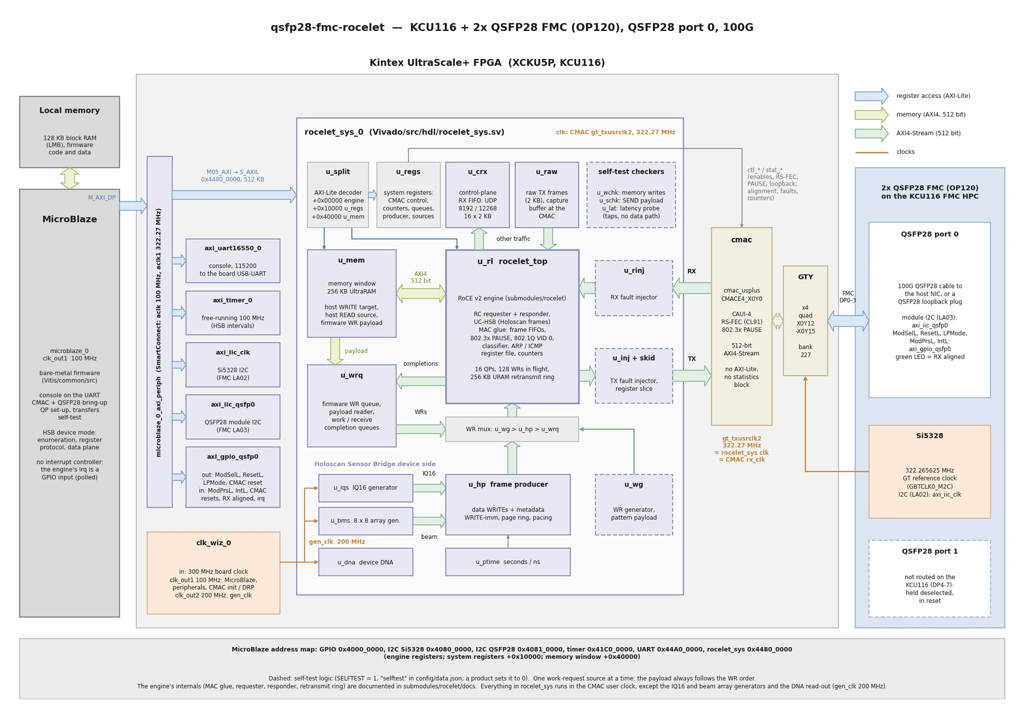
The block diagram below shows the reference design around the engine: the CMAC, a 256 KB UltraRAM memory window for the host’s WRITEs and READs, a MicroBlaze running a UART console for link status, queue pair setup, transfers and counters, optional self-test logic (a line-rate work-request generator, data checkers, fault injectors, a latency probe), and the HSB device side with the array generator. The whole design takes about 55k LUTs, 25 % of the KCU116’s KU5P.

Here are the RDMA results against the ConnectX-6 Dx (3 m DAC, RS-FEC, one queue pair, 64 KB messages, path MTU 4096):

The test host is the bottleneck

The engine runs at line rate in both directions, and unpaced, the board sends 97.6 Gbps of HSB frames. The demo runs at up to 80 Gbps, though, and the reason is the test host. In the P520, the NIC and the GPU sit under different root ports of the CPU, so the NIC’s writes into GPU memory have to cross the CPU’s root complex, on PCIe Gen3. That path tops out at about 81 Gbps, even though the same NIC fills host memory at 97.7 Gbps. A host with the NIC and GPU behind one PCIe switch, or with Gen4/Gen5 slots, should lift that limit, but I haven’t tested one yet.

Within that limit, the results are solid. With every frame compared word for word against the bit-exact model, we saw 0 mismatches at 10, 40, 64 and 80 Gbps, including runs where the stream rate was changed on the fly. A 20 minute soak at 64 Gbps, with the window up, the sources moving and over 20,000 scene changes, put 9.24 million frames into GPU memory with 0 frames lost. The beamforming demo page of the user guide has all the measurements.

Try it yourself

Everything you need to build and run the design is in the user guide. The Getting started page covers the requirements, the build and programming the board, Host setup takes a PC from a bare Ubuntu install to the running demo, and Beamforming demo lists every key, preset and option. If you want plain RDMA transfers instead of the demo, Testing with a host walks through them with the engine’s host tool.

What’s next

I’m planning to experiment with building other Holoscan apps, probably one with our RPi Camera FMC (OP068). I’m also going to get a newer test host, without the P520’s NIC-to-GPU bottleneck, so that I can build something that pushes 2x 100 Gbps through both ports of the 2x QSFP28 FMC (the KCU116 only connects port 0, so that will be on the AMD Versal AI Core VCK190). And I have an idea for combining a RoCE v2 Holoscan app with our FPGA Drive FMC Gen4 (OP063) and a recorder-style design with NVMe offload, like the one in my last post, so that you could record the data you feed into the GPU, play it back, and get the results back out.

Wrap up

Here are the links:

• Reference design: qsfp28-fmc-rocelet on GitHub, and its user guide
• The RoCE v2 engine: rocelet on GitHub, and the rocelet docs
• Datasheet of the 2x QSFP28 FMC, and the Opsero store if you’d like one

I’m pretty happy with how this demo turned out, and -as usual- completely blown away by how quickly I was able to build it and validate it on hardware with the help of Claude Code. I hope the open-source rocelet is useful to a lot of people who need to get data from an FPGA into a host or a GPU. If you build something with it, try it on another board, or have any questions, feel free to reach out or open an issue on GitHub.